Hard Systems Thinking – System Dynamics
System Dynamics (SD) (Forrester, J. W., 1 januari 1958) was developed by Jay W. Forrester of MIT in the late fifties of the past century. This was also the time that computers were coming of age. An important asset of SD is that SD models can be simulated on a computer to get insight in a system’s dynamic behavior by means of “what-if” scenarios. SD was used to underpin the conclusions in the famous publication The Limits to Growth (Donella H. Meadows, Dennis L. Meadows, Jørgen Randers, William W. Behrens III, 1 januari 1972) by the Club of Rome in 1972. This publication showed that growth is limited due to exhaustion of natural resources. The important message was that our way of (western) life is unsustainable. Remarkably, the predictions turned out to be mostly true.
The structure of a system is determined by its elements and the relations between its elements. The inter-connectedness between elements amounts to that one element can have an effect on other elements, and so on. In this way, a system shows its behavior in the form of actions and reactions of elements. System Dynamics (SD) captures the dynamics by showing how changes in the key characteristics of elements have an effect on other elements’ characteristics. In SD jargon, the characteristics are called variables.
The research philosophy that corresponds with SD is positivism.
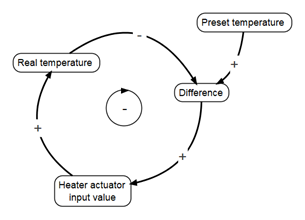
Using the thermostat as an example again, the corresponding SD model is shown below.
The variables are connected to each other with an indication of how a target variable changes as a result of a change in a source variable. The plus sign indicates that a change in a source variable induces a change in the same direction in the target variable, likewise a minus sign means a change in the opposite direction. The inclusion of a minus relation in the loop makes it a negative feedback loop, also known as a Balancing (B) loop, as is visually accentuated in the middle of the loop with the circle with an arrow containing the minus sign. Because loops play a key role, a SD model is frequently called a Causal Loop Diagram (CLD).
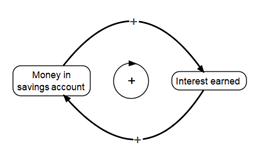
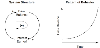
An example of a positive feedback loop, also called a Reinforcement (R) loop, is shown below. It shows how money in a savings account exponentially grows because periodically the savings are incremented with interest earned over the savings, provided the interest rate is positive. But nowadays, we are facing negative interest rates. In that case, the system still has a positive feedback loop, but unfortunately, the savings decrease exponentially.
Een alternatief dat de groei laat zien.
SD was further popularized by Peter Senge in the Fifth Discipline (Peter M. Senge, 6 april 2006). He showed that archetypal patterns are at work as undercurrents in organizations. Frequently, wanted or unwanted results are often diagnosed for the wrong reasons because the effects of balancing and reinforcing loops behind the scene are overlooked. Recognizing the archetypal patterns at work helps to avoid making the same mistakes time and again.
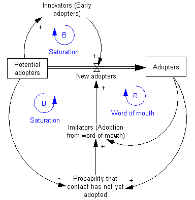
A somewhat more complex example is shown below. It is a model of how a product is adopted by customers. The model contains three interacting loops, of which two are of the balancing kind (B) and the remaining one is a reinforcing (R) loop. Two new modeling elements are included in this example: stock and flow. A stock is a reservoir in which all kind of things can be inserted and retrieved. This example features two stocks containing adopters and potential adopters. The goal is to turn a potential adopter in a real adopter. That is, to move a person from one stock to another. This transfer is modeled as a flow, and the flow rate can be influenced by all kind of factors, including … If a product is increasingly adopted and the adopters are satisfied with the product, the increase in the positive “word of mouth” feedback increases the adoption flow rate. However, as more and more potential adopters are turned over, the potential adopter stock is running dry. This has of course a negative effect on the turn-over flow rate. So, after an initial adoption rate rise, the adoption process gradually comes to an end because of lack of potential adopters.
Opmerking: Een combinatie van deze twee maken.
Statement: A system comprised of a number of interacting feedback loops is a complex system whose behavior can surprise us.
Aspect: Systems Thinking, Principle: Create room for change, Principle page: Principles and Ground Rules
| Statement page | Statement |
|---|---|
| Hard Systems Thinking – System Dynamics | A system comprised of a number of interacting feedback loops is a complex system whose behavior can surprise us. |
| Systems Thinking | A system as a whole is comprised of parts. Systems thinking is about understanding the interactions between the parts. |
Principles, aspects and statements overview
- Create room for change, defined in page: Principles and Ground Rules
- Systems Thinking, defined in page: Principles and Ground Rules
- Hard Systems Thinking – System Dynamics (A system comprised of a number of interacting feedback loops is a complex system whose behavior can surprise us.)
- Systems Thinking (A system as a whole is comprised of parts. Systems thinking is about understanding the interactions between the parts.)
- Critical Reflection, defined in page: Principles and Ground Rules
- Determining Boundary Judgements with CSH (A constructive dialog can take place on the basis of first and second order boundary judgments.)
- Self-observation (Concentrate on how to look, instead of what to see.)
- Self-observation (You need someone else to point out your blind spots to you.)
- Diversity in opinions, defined in page: Principles and Ground Rules
- Worldview, defined in page: Principles and Ground Rules
- Model Building - Human Activity Systems (A worldview (Weltanschauung) captures the beliefs, desires and intentions of a person.)
- Model Building - Human Activity Systems (The PQR formula (what, how, why) is pivotal for capturing worldviews.)
- Soft Systems Thinking – Soft Systems Methodology (People differ in worldviews, but nevertheless they typically adhere to aspects of multiple worldviews, which provides room for accommodation.)
- We got to move, defined in page: Principles and Ground Rules
- Reflexive Domain, defined in page: Principles and Ground Rules
- Exploring Change (The constant factor in life is movement.)
- Self-Reference in a Three-Valued System (Embrace the paradox, i.e., a difference in what was previously stated and therefore contradicting what was said before. Differences keep setting things in motion. Without differences we cease to exist. Therefore, change is inevitable, in fact, it is a necessity for living.)
- The Autopoietic Turn (Humans and social systems operate autonomously and my react when irritated.)
- Tradition, defined in page: Principles and Ground Rules
- Exploring Change (A system has to become what it is not, and yet remain the same.)
- Some-thing from No-thing (The relationship between things, including humans, is what matters. Something or someone cannot stand or be taken on its own.)
- Determine the right direction, defined in page: Principles and Ground Rules
- Cultural Identity, defined in page: Principles and Ground Rules
- Investigating Identity (Group identity refers to a person’s sense of belonging to a particular group.)
- Research Philosophy and Process (Research approach must be “for you, and with you”, instead of “for you, but not with you”.)
- Right Things, defined in page: Principles and Ground Rules
- Co-dependency, defined in page: Principles and Ground Rules
- Ethics of Care, defined in page: Principles and Ground Rules
- Investigating Identity (Ethics of Care is a retreat to first principles to be part of a group to protect and to provide meaning.)
- Responsible Setting for Social Innovation (Each stakeholder facilitates other stakeholders in addressing a societal challenge.)
- Some-thing from No-thing (We rely on each other and therefore we should care for each other.)
A system comprised of interacting loops is almost by definition a complex system whose behavior is difficult to understand and to predict. Reinforcing feedback loops imply exponential growths that must be somehow tamed with balancing feedback loops. The challenge is to find the sweet spot where the system stabilizes at desired levels in time and is able to absorb disruptions. The complexity can be overwhelming, and for that reason, SD models are simulated to assess their dynamic behavior.


